THE STRUCTURE OF THE BRAIN
AND OF THE ADAPTIVE
COMPUTER ARCHITECTURES
Department of Computer Science
St. Catharines, Ontario
Canada L2S 3A1
January 1998
ABSTRACT
The goal of this paper is to describe ways to create systems that would use their experience of past executions of algorithms in order to improve automatically their own performance in terms of speedup. Described are the mechanisms for detecting available parallelism in algorithms and methods of search for and classification of optimal processor configurations. Analogies between the computer and biological systems are suggested.
NOTE: The mathematical notation presented is best viewed using Internet Explorer 4.01 or later.
DREAMS, EVOLUTION AND PARALLEL PROCESSING
The ever-growing need for more and more powerful computers is universally evident. Similarly recognized are the impressive developments in computing technology. If we were to attribute these developments to a single motivating factor, this factor could arguably be our ever-growing need for computational speed.
The R&D efforts aimed at the development of uniprocessors are well established, focused, and, so far, regularly productive, in terms of offering technically sound and financially feasible solutions.
A similar statement with regard to the development of multiprocessors cannot be made with equal confidence. The technological limits of the uniprocessor technology, dictated by the laws of physics, are universally recognized, thus offering the incentive to get us interested in parallel processing. Sadly, the implications of the conceptual limits, imposed by logic, tend to dampen our enthusiasm.
The most important conceptual limit is arguably the halting program theorem. It states that it is impossible to construct an algorithm capable of determining whether an arbitrary program, operating on arbitrary data, would halt or not. Consequently, it is therefore impossible to write a program that would estimate the execution times of other programs, operating on given data, without actually executing these programs. After all, the unanswerable question whether an arbitrary program halts is a special case of a more general question: How long does it run?
What has been said about arbitrary programs applies as well to arbitrary subprograms, dimming our hopes that application of parallel processing will prove to be a simple solution to our quest for ever greater computational speed. After all, our initial motivating impulse was to allocate the subprograms of a given application program to various processors, with hope that the resulting configuration would execute successfully and faster than on a uniprocessor.
The widely recognized difficulty with this approach is that there are many ways of splitting a program into subprograms. Then, for each such split, there are many ways to allocate processors to the subprograms. Some of these allocations will be superior, in terms of execution speed. Some of them might perform worse than the simple execution of the entire program on a uniprocessor.
How then are we to perform this search for optimal processor allocation? Manual search is out of the question. The search cannot be easily automated using some smart compiler technology that would somehow produce optimally allocated executable codes: compilers do not execute the programs, but only transform them into other programs, that are equivalent, from some point of view. Therefore, compilers cannot compare execution times of various allocations.
Is then such search feasible and practical? Not to those sporadic users who want to run an application program only once for a given set of input data, obtain the result, and then return to their main activity. As to the feasibility: it will be evident a bit later that given the current state of computing technology a brute force search for optimal processor allocation for most commercial algorithms would take longer than the age of the Universe. However, a user routinely executing the same program with a given set of input data might be an interested in owning a program that would use its own execution experiences to keep configuring the computer on which it runs and reallocating itself to run ever faster.
Keeping all these difficulties and promises in mind, we still do a lot of research on parallel computing, the preferred architectures being processor pipelines, meshes of trees, hypercubes, symmetric multiprocessors, etc. Most researchers seem to be preoccupied with the following problem:
We sometimes get the uneasy feeling that we are doing it backwards. Computers were supposed to be tools, after all! Therefore, the proper problem seems to be:
The goal of this paper is to suggest a way to create programs that would use their experience of past executions in order to improve automatically their processor allocation. The proposed solution, while feasible and hopefully elegant, will by no means be technologically simple. Please note that two different sets of runs of the same program, performed by two users, with possibly different data sets, may call for a different number of processors differently interconnected, if speedup is to be maximized. How then can we know a priori the optimal computer architecture to run a given algorithm? We simply cannot. Indeed, such a fixed architecture may not exist.
We can, however, perform an adaptive search for optimal processor allocation independently at each user site. We will take our clues from Nature.
Nature manages to evolve systems capable of ever-speedier computational feats. (Evolve is the term biologists would use; computer scientists are likely to prefer the term search). For example: At some stage the early primates learned to throw stones in fights and hunts. If our survival depended on the acquired abilities to recognize and evade flying stones, then our skills of recognizing such airborne objects and forecasting their trajectories were only useful if we could execute the necessary algorithms before the obvious deadlines. The primates unable to meet the deadlines (of this and other nature) were removed from the environment. The search continues.
Biologists and psychologists frequently use the terms like evolution, brain, consciousness, dreams, etc. While their work has put us on the proper track in our efforts to maximize algorithm execution speed, these terms lack sufficiently precise meaning to be of direct use in computer science. For the purpose of this work, we therefore define:
Brain: an ordered pair of two interconnected multiprocessor computers. The first computer is dedicated to run algorithms needed by the user, while the second computer gathers the timing information and input data of the algorithm runs performed by the first computer. This information will be used subsequently by the second computer to fine-tune the architecture of the first computer. Obviously, when the first computer is subject to the tune-up, it cannot be available to the user. (The biologists would then say that the user sleeps). The second computer is never directly available to the user.
Alertness: the period of time when the first computer is available to its user. (The biologists would say that its user is awake). During this period the second computer gathers the timing information and the input data for the algorithms run by the first computer.
Sleep: the period of time when the architecture of the first computer is being reconfigured by the second computer, the first computer being unavailable to its user.
Dreams: acts of execution of user's algorithms for the purpose of obtaining timing information rather than providing user with the result. Such executions try out various processor configurations. The input data are identical to those used by the alert user.
Obviously, the above definitions, especially the one of the brain, would make most psychologists shudder. We will use them only as useful abstractions of more complex objects and ideas.
Our strategy will rely on our luck to live in an environment that is predictable to some extent. The changes that happen in it happen sufficiently slowly, so that we can manage to reconfigure our computer brains in order to maximize speedup (or, at least, to keep up with the environment). Let us take the weather for example. It turns out that the reliability of the simple forecast: The weather of tomorrow will be much like the weather of today is close to the best forecasting methods ever designed. In order to be able to come up with even more reliable forecasts (among others) we perform our brain reconfigurations on the fly. The brains we use today were configured last night using the input data of yesterday. Lucky for us, this configuration is close enough to the optimal one, and this night we will refine it, in order to keep up with the environment of tomorrow.
SEARCH FOR OPTIMAL COMPUTER ARCHITECTURE
As we have said, given the current state of computing technology, brute force search for optimal processor allocation for most commercial algorithms would take longer than the age of the Universe. Let us justify this statement and suggest a more intelligent search strategy. First, let us establish some nomenclature:
Algorithm: a finite sequence of instructions designed to provide a solution to the problem at hand within the required accuracy. When executed, it is required to reach the solution within a finite number of steps and is allowed to require only a finite amount of computational resources (time, memory, processors, etc.). Also called: a program.
Process: an act of single execution of an algorithm, with one input datum. In a given computer we may have a number of processes executing the same algorithm, typically with different input data (compilations, text editing sessions, device drivers, etc.).
Task: a single thread of execution. A process may consist of several cooperating tasks.
In other words, an algorithm a is a function:
a : D � R
operating from some set of input data D (also called domain of algorithm a) onto some set of results R (also called its range). We will also require that for at least one element d � D the algorithm a halts, i.e. its program produce some result r � R within finite number of steps. In short, we have required for the algorithm to be devoid of deadlock and livelock for at least one element d � D. Indeed, there may be (and hopefully is) a subset D � D for which the algorithm a halts. The trouble is, that according to the halting problem theorem, there is no algorithmic way to identify D within D.
Initially, we ensure experimentally that the algorithm a halts for at least one datum d � D, by writing, debugging and editing its program until it is forced to halt. A program may consist of several cooperating tasks. In current programming languages, each task is fired by a system call of the kind:
FORK (<task_id>, <startup_info>);
where <task_id> is typically a subprogram identifier, while <startup_info> contains auxiliary operating system instructions.
Consequently, it is possible to uniquely identify the tasks fired as the program executes. Let us consider the task T0 to be the main program. Then we start counting tasks being fired by counting the instances of execution of the FORK system call.
Consider a program executing the algorithm a with input datum d � D, consisting of n tasks T0, T1, T2,..., Tn-1. We will search for the optimal processor allocation, minimizing the execution time.
To say that we know that this program consists of n tasks, is to say that we have successfully executed it to a halt (perhaps on a uniprocessor, interleaving its tasks), using a particular input datum. In that case we could have noted not only its result r, but also its execution time tex. We will compare all possible processor allocations, considering tex as our deadline. Alternatively, we could have picked as the deadline any other value tdead, imposed on us by the environment (customer specification, benchmark requirement, etc.). In our search we will not be interested in processor allocations resulting in the execution time exceeding our deadline. Indeed, in such cases we will not bother to run our program to completion. We will just abort it when the deadline expires.
Obviously, the speed of execution depends on the hardware at our disposal. Suppose we have a computer with m processors P0, P1, P2,..., Pm-1. In general, these processors may have different characteristics (speed, word length, various amounts of on-chip memory, instruction set, etc.) We will keep allocating these processors to our tasks. The cooperation between tasks implies intertask synchronization and communication. In order not to sacrifice all the elegance of the advances in the machine independence, afforded to us by software engineering, we need to augment the FORK system call to:
FORK (<task_id>, <processor_id>, <startup_info>);
Using this new system call we will be able to explicitly assign a specified processor to a given task. Another system call will be needed to establish unbuffered, unidirectional logical links between two tasks, which may run on two different processors:
LINK (<source_task_id>, <target_task_id>);
Obviously, when using the LINK system call we can create bi-directional links by using two unidirectional links of opposite orientation. Similarly, with a little bit of programming effort, we can establish buffered links.
The bandwidth of these links will no doubt depend on the characteristics of the underlying hardware connection. In particular, the architecture of the computer at hand may not allow establishing a link between a particular pair of processors Px and Py. In this paper we will not treat this situation as a special case. Rather, we will assume that the established link has bandwidth zero. Cooperating tasks using this particular link will not be able to complete so that the overall program meets the deadline tdead. In short, we assume that the execution of the LINK system call never fails.
Another reason for our program not meeting the deadline tdead might be the allocation of one of its tasks, say, Ti, to a processor Pk incapable of executing one of the instructions of code of Ti because the offending instruction is not in the processor's instruction set. We will assume then that the processor Pk hangs up, thus preventing the overall program to meet the deadline. We could, if we wanted to, prevent such a situation from happening, by scanning all the instructions forming the code of Ti and checking that they all are within the instruction set of Pk.
We will not follow this approach, however, because it is too strict. The code of the task Ti, apart from the offending instruction, may contain some conditional branch (i.e. IF) statements. There is no general way of knowing, which branch of the IF statement code (if any) the execution will follow, when our program is executed using the input datum d. Chances are, the section of code of Ti containing the offending statement may be bypassed entirely. For special cases this approach is not without merit, however.
In general, given the program with n tasks and the computer with m processors, there are a priori mn possible processor allocations. To illustrate this, consider all possible allocations of a two-task program on a computer of three processors. The possible allocations are listed in Table 1 below. The tasks are numbered 0 and 1, the processors are numbered 0 through 2.
Allocation  Task 1  Task 2
    #
    0         0       0
    1         0	      1
    2         0	      2
    3         1	      0
    4         1	      1
    5         1       2
    6         2	      0
    7         2	      1
    8         2	      2
Table 1. Possible allocations of a two-task program for a computer of three processors.
The first column of this table indicates the allocation number (0 through 8, 9 allocations in total; 9=32), the second and the third columns indicate the processor numbers allocated to task 1 and task 2 correspondingly.
The NP-completeness of the processor allocation problem should not frighten us exceedingly. NP-complete problems are hard when attacked using uniprocessors. Most of them lend themselves to an easy treatment on parallel computers.
To illustrate this, consider the above example. Suppose that all three processors have different characteristics. If we had a computer with 27 processors, 9 of them of type 1, 9 of type 2, and 9 of type 3, we could try out all possible 9 allocations simultaneously. The whole allocation search experiment would last at most tdead time.
Granted, for nontrivial applications such a parallel search approach requires big multiprocessors. No wonder that the brain, consisting of 100 billion neurons, comes to mind.
Fortunately, it will be rather infrequent that an application will require many processors of different types. Suppose that in the former example the processors 1 and 2 are identical. Suddenly, the number of possible allocations collapses dramatically. The allocations 1 and 2 become identical and it is enough to try out only one of them. Similarly, the allocations number 3 and 6 require testing of only one of them, and again the same goes for allocations 4, 5, 7 and 8. In total, we need to test four allocations instead of nine. The larger the application program, the larger the potential savings. Indeed, it would be ideal to utilize one type of processors only. As the studies of theory of computation indicate ([Davis and Weyuker, 1983], [Boolos and Jeffrey, 1987], [Epstein and Carnielli, 1989]), it turns out to be possible. It is no accident, therefore, that the human brain is made of processing elements of fundamentally one type (neurons).
Using our newly established terminology, the trial allocations are dreams. Indeed, one might suggest that the whole period of sleep consists of two subperiods: the first being the period of dreams, the other being the period of the reconfiguration of the user computer, in order to reflect the identified optimal architecture.
These suggestions, although correct, are premature at this point. We have just run our program for one datum d. Another execution, for a different input value, may result in a different number of tasks being fired, and require a different optimal architecture.
It is hard, however, to resist the temptation to go a bit further and offer some tentative suggestions of implementation, at least for simple algorithms that use relatively few optimal architectures. We should avoid executing the LINK system calls at alert time on the user computer - their execution wastes time. Instead, we could prelink all the recognized optimal architectures for a given algorithm in the user computer and execute the algorithm on all of them simultaneously. As soon as the execution of one of these processes terminates, we offer the user the result and abort the processes running on different processor architectures.
To justify the correctness of these suggestions we must first establish a mechanism capable of recognizing potential parallelism in algorithms, and then propose a method for classifying emerging optimal architectures. Only then we could viably offer our suggestions for the implementation of computers with adaptive architectures.
We will do just that.
AUTOMATIC RECOGNITION OF PARALLELISM IN ALGORITHMS
The concepts of algorithm and language are intertwined. An algorithm does not exist until it is written. Having written it down, we have implicitly chosen some language. Every language inhibits to some degree our capabilities of expression. We strive to design languages, which enforce as few such limitations as possible. It is impossible, however, to design a language in which all the algorithms, even those yet to be invented, are expressible. It looks therefore that the developments of linguistics and algorithms will proceed in parallel forever.
Neither an algorithm nor a language can exist without the existence of a computer. The converse is also true. The developments in computer technology, linguistics and algorithm design stimulate each other. In this paper we will not dwell on this fascinating subject. Let us only point out that we are not describing vicious circles, but rather three arms of an unveiling, evolutionary spiral.
The reason that we mentioned this subject at all is because we have recognized the need for languages capable of highlighting the inherent parallelism in algorithms. Not all expressions of the algorithm as an implementation of the function
a : D � R
are equivalent, in terms of the inherent possible parallelism. Indeed, an algorithm a could be considered a member of a larger set A of all possible expressions of the above function in all existing languages. It is the job of compilers to perform the necessary program transformations. We are interested in possible expressions that maximize the parallelism potential. Compilers also transform algorithms to fit the particular features of an underlying machine. Strictly speaking, machine independence is a fiction, albeit sometimes a very useful fiction.
The programming languages currently in use tend to suppress the evidence of parallelism in the algorithms they describe, therefore damaging the inherent structure of algorithms. A possible noble exception is OCCAM 2, a programming language in which it is possible to algorithmically undo such damages. Interested readers are directed to [Hoare, 1985], [INMOS, 1988], [Roscoe and Hoare, 1986], or, for a quick overview to [Burns, 1988]. Luckily, the researchers in compiler technology start to recognize current linguistic deficiencies.
For the purpose of this paper we will assume now that we have at our disposal an implementation of the algorithm a with sufficient inherent parallelism. At the end of this section an algorithmic criterion for recognizing such parallel implementations will emerge.
Let us study the acts of execution of algorithms, with the intent of representing them as graphs. An executing algorithm, using some input datum, performs a number of operations, then halts. Let us represent these operations as nodes in our graphs. An operation may require some data as input, and may produce some results as output. For an operation requiring some input data we will draw arcs directed to the node representing that operation, the number of arcs being equal to the number of input data. Similarly, if an operation produces some result(s), we will draw arc(s) originating at the corresponding node and directed away from the node. If a given datum, required by some operation is produced by another operation, we will link the nodes representing the producer and consumer operations with an arc directed form the producer to the consumer node.
Please note that in a graph so created, some arcs may not originate at any node. Similarly, there may be arcs pointing to no node at all. Such arcs will represent the program input and output data, correspondingly. We will call them the input and output arcs.
The graphs so constructed will be called algorithm graphs. Observe that the shape of the algorithm graph (number of nodes and their interconnections) may change if we execute the same algorithm for various data d � D from its domain. However, any algorithm is uniquely represented by the set of its algorithm graphs for those input data d � D, for which the algorithm halts.
Let us study the properties of the algorithm graphs rather than the algorithms themselves, with the intent of detecting a possible parallelism. Let us remove the input and output arcs, and observe the properties of the resulting directed, acyclic multigraphs.
THEOREM 1. Any directed, acyclic graph with a finite number of nodes contains at least one node to which no arcs point and at least one node from which no arcs originate.
PROOF. This is obviously true for graphs containing no arcs. Suppose then that a graph contains at least one arc. Consider a starting node of any critical path in this graph. Suppose that there is an arc pointing to it. We may have two situations here:
- The node from which the arc originates belongs to the critical path. In that case we have found a circuit in our acyclic graph, contrary to our assumptions.
- The node from which the arc originates does not belong to the critical path. In that case we have found a path longer than the critical path, ending again in a contradiction.
Therefore, a starting node of any critical path in our graph is the node to which no arcs point. Similarly, it can be proven that the ending node of any critical path in our graph is the node from which no arcs originate.
Q.E.D.
The theorem we have just proved permits us to arrange the nodes of our graph into three groups: the starting nodes, the internal nodes and the final nodes. If a critical path has a length of 2 or more, none of the three groups is empty. This node grouping amounts to the detection of a crude parallelism: all operations represented by the starting nodes could be executed in parallel, followed by similarly parallel execution of all operations represented as internal nodes, and terminating by the parallel execution of all operations depicted by the final nodes.
This finding may not be sufficient. We want to explore the entire parallelism that is hidden in our graph. Consider:
THEOREM 2. All nodes in an acyclic, directed graph of n nodes can be labeled with integers from {1, 2,..., s}, where s�n so that if an arc points from a node labeled with i to a node labeled with j then i<j.
PROOF. Consider all nodes to which no arcs point in the graph. Label them with 1 and remove them from the graph, together with arcs originating from these nodes. The resulting graph remains an acyclic, directed graph. Repeat the same exercise labeling all removed nodes with 2. Continue this procedure, until the whole graph is disassembled. The number of steps s this procedure is executed cannot exceed n, since each time we have removed at least one node.
Q.E.D.
The described labeling procedure of all nodes in our graph is called the strong topological sorting of a graph, or topological sorting, in short. This sorting permits us to detect the entire parallelism available in the graph. Obviously, all operations represented by nodes labeled with 1 can be executed as tasks in parallel, followed by all operations indicated by nodes labeled 2, etc. This is so because no nodes with identical labeling are connected with a producer/consumer arc.
For every graph we can identify the largest group of identically labeled nodes. Let us define the graph width to be equal to the number of nodes of that group. In the same vein, we can define the algorithm width as the maximum of the widths of all the graphs describing given algorithm.
Similarly, for every graph we can define its height as the length of the critical path plus one. By algorithm height we will understand the height of its tallest graph.
Earlier in this section we suggested an emergence of an algorithmic criterion for distinguishing between inferior and superior parallel implementations of algorithms. As we have said, each algorithm implementation corresponds to a family of algorithm graphs. Good parallel implementations will have a high algorithm width and a low algorithm height.
In future computer systems we would like to treat pools of processors as a fluid computational resource, much like we treat pages in paged virtual memory management systems now. Users should be free to dynamically draw processors from the pool and return them after use. The trouble with this approach (apart from the financial aspect) is that users have difficulty answering the following question:
The answer: the number of processors in use will fluctuate during execution, but the algorithm width is its upper bound.
At this point of our analysis we may begin to worry that, in terms of the detected parallelism, we detected too much to handle. Certainly, keeping with modern programming strategies, we would like to exploit the parallelism in steps. We would like to analyze a conveniently small part of the available parallelism at any given time, deferring the analysis of the rest. To do that, we need a so called weak topological sorting of our graph, defined by the following:
THEOREM 3. All nodes in an acyclic, directed graph of n nodes can be labeled with integers from {1, 2,..., s}, where s�n so that if an arc points from a node labeled with i to a node labeled with j then i�j.
PROOF. The proof is identical to the proof of theorem 2.
Q.E.D.
Such labeling of nodes in our graph allows us to organize the nodes into groups, but this time we are allowed to leave some sequential interdependencies between some operations belonging to the same group. This permits us to exploit the parallelism in an algorithm, perhaps at some procedure level, delaying the exploitation of parallelism in these procedures.
CLASSIFICATION OF OPTIMAL ARCHITECTURES
Given the algorithm a, the optimal processor allocation depends on the data point d � D, for which its program is executed. The search for this allocation, while not brute force, must scan (at least partially) a vast number of configurations. This implies that the second computer of the brain, the one never directly available to the user, must be much larger than the first computer. This observation suggests the answer to the puzzle perplexing the physiologists for some time. They wonder why the brain seems to violate the rules of the superbly efficient and parsimonious design of the human body. According to their estimates, we use approx. 5 to 10 per cent of our brain capacity. What is the remaining part for, and why did it not waste away if it is not in continuous use? The answer seems to be: it is in continuous use, but mainly at sleep time, searching for optimal processor allocations for a number of algorithms, and, for each algorithm, for many input data points.
For our algorithm a we do not need to know all optimal processor allocations for every datum d � D, but only for these values that the user encountered or is to encounter at alert time. Indeed, we have reasons to suspect that the distribution of probability of a given datum being encountered is not uniform over the set D.
We can think of the optimal computer architecture as a function f(d) of data points. Informally, the number of optimal configurations will be smaller than the number of data points. One could even argue that the number of elements in D is finite, although very large: every processor, having a fixed word length, can represent only a finite number of different values. Sensors, providing input data from the environment can be considered processors. An alternate argument: we inhabit an environment that is of quantum nature, and our sensors have some ranges of operation. Therefore, we can perceive only a finite number of input data values. In this paper we will not need the assumption of the finiteness of D. However:
THEOREM 4: The number of optimal configurations to be stored in our computer is finite.
PROOF. Having performed a finite number of runs for given input data values, we can come up with at most finite number of configurations, one for each run.
Q.E.D.
It is quite possible for two different data points x, y � D to obtain identical architectures f(x) = f(y). We say then that points x and y are equivalent. We expect to see regions in D such that all input data from each region call for the same multiprocessor architecture. We could run some pattern recognition programs to identify these regions. After some experience has been gathered, we might try to guess the region to which new and untested data points belong. This exercise could be performed both at sleep time and at alert time. Our current successes with computer systems equipped with the virtual memory management mechanisms provide sufficient motivation to try out this idea.
To formalize this approach, let us consider a relation of equivalence E over the set D. For x, y � D we will write xEy if and only if f(x) = f(y). Relations of equivalence have the following properties:
(i) ("x � D) xEx
(ii) ("x, y � D) if xEy then yEx
(iii) ("x, y, z � D) if xEy and yEz then xEz
These properties are known as the reflexive, symmetric and transitive laws of any equivalence relation.
Let us further define:
Quotient map: Let E be an equivalence relation in D. Let further P(D) be a powerset of D, i.e. the set of all subsets of D. The quotient map associated with E is the function:
j : D � P(D) with values defined by j(x) = {y | xEy}
The quotient map is also called natural map. The various sets j(x) are called equivalence classes of E. The set of all equivalence classes, i.e. the range of j, is called the quotient set of D by E. A member of an equivalence class is often called the representative of the class.
Finally, let us define:
Partition: a partition P of the set D is a collection of nonempty subsets of D such that for each d � D there is exactly one B � P with d � B.
In other words, P is an exhaustive collection of mutually exclusive subsets of D.
Our cognitive exercise of learning the properties of the partition of D that would reflect the optimal processor architectures is based on the following theorem, well known to the mathematicians specializing in abstract analysis, which we will give here without proof:
THEOREM 5. Let E be an equivalence relation in D, and let Q be the quotient set of D by E. Then Q is a partition of D. Conversely, if P is any partition of D, then there is a unique equivalence relation F in D having P as its quotient set.
Readers interested in the details of the proof might peruse [Gleason, 1991], or any other book on abstract analysis.
IMPLEMENTATION CONSIDERATIONS
Although we are generally interested in the computational speed, let us focus on the operation of the real time systems, biological or otherwise. In these systems, obtaining results within deadlines is of paramount importance. Since it is always possible to formulate a deadline impossible to meet, we will therefore consider only 'practical' deadlines, i.e. deadlines for which feasible multiprocessor architectures exist.
The fastest way of implementing an algorithm is to store the results of computation in a table, indexed by the argument values. The table should be created at sleep time and accessed in parallel at alert time. This is how the mathematicians define a function: as a set of ordered pairs. If this maximally parallel approach will not enable us to meet the deadline, no other software approach will. The only hope left is in the performance improvements of hardware technology.
Unfortunately, due to substantial cost and memory limitations this method is feasible only for algorithms with very small domains or for selected argument values. The utilization of PARs (page address registers) in virtual memory management systems could be an example of its successful application.
The next best thing is to store all optimal architectures for the algorithm and use them in parallel to obtain the result. As soon as it is obtained on one of the architectures, the processes running on other architectures are aborted.
This approach is guaranteed to work (assuming 'practical' deadlines) only for simple algorithms, where it is easy to identify the proper partitioning of the algorithm's domain, and where the number of the equivalence classes is sufficiently small so that we can simultaneously store all the optimal architectures, one for each equivalence class.
What if we cannot meet these storage requirements? This situation can arise for nontrivial algorithms. It almost certainly arises in the case of the human brain, which runs a vast number of nontrivial algorithms.
Suppose we are to run a nontrivial algorithm for the first time. We have no idea how many optimal architectures there might be and what is the one for the current datum. We can run the algorithm on a uniprocessor. This will probably make us miss the deadline, but at least we will be able to recognize the algorithm graph. If we have a vast number of randomly connected processors, it will not hurt to initiate simultaneously the execution of this algorithm in a number of places in the network. Each such process we will delegate the emerging parallel operations to other processors along the existing hardware links. This does not guarantee success, but the larger the network and the denser the interconnection mesh, the more such processes we can fire, and the higher therefore is the probability that one of these processes will not hang up, and perhaps even meet the deadline. In any case, we do not expect spectacular performance during the first alert period.
During the first period of sleep, we will fine-tune the processor allocations by identifying architectures for the newly recognized algorithm graphs. The best allocation would assign a separate processor to each operation represented by the node in the graph. For small multiprocessors this may not be practical, in terms of the number of processors needed. A good allocation does not serialize operations that could be executed in parallel. In terms of topologically sorted algorithm graphs, a single processor allocation is a subset of nodes in the graph such that no two nodes have identical label. The operations represented by nodes listed in an allocation are not intended to be executed in parallel. The architecture is the set of allocations such that each graph node is listed in one allocation only, and no nodes are omitted. If the processors available were at a premium, the architecture of interest would contain the smallest number of allocations.
Unfortunately, the algorithm graphs detect only the inherent parallelism between operations, but contain no information concerning the time needed to execute various operations. This is why the dreams come in... A compromise is needed between the most parsimonious architecture (in terms of the number of processors used) and the fastest. The compromise architecture is the most parsimonious among those, which are able to meet the deadline.
As time passes and the sleep and alert periods alternate, we continue to enrich our library of selected architectures. The real time performance of our algorithm improves, but we may approach the limits of storage capacity, in terms of the number of architectures. We may be interested in reducing the number of architectures by giving up those, which have not been in use for a long time. This is typically done in the assumption that the environment changed, so that these architectures are of lesser value now. We certainly observe the reduction of non-refreshed skills in humans.
Earlier in this section we have recognized the benefits of including in the user computer the largest possible network of processors with the biggest number of interconnections, technology permitting. These benefits obviously apply to the second computer of the brain as well. As an added bonus, our artificial brain can attain the seemingly miraculous capability of self-repair: in some cases it will be possible to reconstruct lost information regarding the identified optimal processor architectures.
In the long run, in a relatively stable environment, the user part of the brain will be required to run a relatively unchanging mix of algorithms, and the architecture optimization searches will yield diminishing returns. The user part of the brain will become very efficient but highly specialized: it will be able to execute certain functions only, much like a real-time controller in an industrial setting. We could say that it loses its intelligence.
A subsequent change in the environment will require running new algorithms, for which our biological real-time controller will be ill suited. The only solution is to leave it alone doing what it is good at, and to divide the remaining part of the brain into two regions: the first, accessible to the user, and the second, optimizing the performance of the first region.
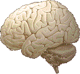
The anatomy of the brain reflects this progress of evolution through punctuated equilibria. At the first glance we can easily identify three different regions: the brainstem, the cerebellum and the cerebrum. The brainstem, the smallest of the three, is responsible for controlling the most ancient body functions like breathing and digestion. The larger cerebellum is controlling more recent but still routine functions, like maintaining posture and controlling body movements. The largest of the three regions, the cerebellum, consisting of two hemispheres linked by the corpus callosum, is the site of our conscious and intelligent activities.
Coming back to the realm of computer science, let us paraphrase our definition of the brain: it is a large network of vastly interconnected multiprocessors. One part of the network is allocated to run user algorithms, while the other part optimizes the performance of the first part. The demarcation line, defining where the user part of the brain ends and the optimizing part begins, has always been left completely arbitrary. As the overall size of the network grows, the demarcation line might move and the newly defined brain would start optimizing certain new algorithms, perhaps including some of the old optimization routines.
The evolution continues.
REFERENCES